Sine-squared function

This article is about a particular function from a subset of the real numbers to the real numbers. Information about the function, including its domain, range, and key data relating to graphing, differentiation, and integration, is presented in the article.
View a complete list of particular functions on this wiki

Definition

This function, denoted $\sin ^{2}$, is defined as the composite of the square function and the sine function. Explicitly, it is the map:

$x\mapsto (\sin x)^{2}$

For brevity, we write $(\sin x)^{2}$ as $\sin ^{2}x$.

Key data

Item	Value
Default domain	all real numbers, i.e., all of $\mathbb {R}$
range	$[0,1]$, i.e., $\{y\mid 0\leq y\leq 1\}$ absolute maximum value: 1, absolute minimum value: 0
period	$\pi$, i.e., $180\,^{\circ }$
local maximum value and points of attainment	All local maximum values are equal to 1, and are attained at odd integer multiples of $\pi /2$.
local minimum value and points of attainment	All local minimum values are equal to 0, and are attained at integer multiples of $\pi$.
points of inflection (both coordinates)	odd multiples of $\pi /4$, with value 1/2 at each point.
derivative	$x\mapsto \sin(2x)=2\sin x\cos x$, i.e., double-angle sine function.
second derivative	$x\mapsto -2\cos(2x)$
$n^{th}$ derivative	$2^{n-1}$ times an expression that is $\pm \sin$ or $\pm \cos$ of $2x$, depending on the remainder of $n$ mod $4$
antiderivative	$x\mapsto {\frac {x}{2}}-{\frac {\sin(2x)}{4}}+C$
mean value over a period	1/2
expression as a sinusoidal function plus a constant function	$(1/2)-\cos(2x)/2$
important symmetries	even function (follows from composite of even function with odd function is even, the square function being even, and the sine function being odd) more generally, miror symmetry about any vertical line of the form $x=n\pi /2$, $n$ an integer. Also, half turn symmetry about all points of the form $(n\pi /2+\pi /4,1/2)$.
interval description based on increase/decrease and concave up/down	For each integer $n$, the interval from $n\pi$ to $(n+1)\pi$ is subdivided into four pieces: $(n\pi ,n\pi +\pi /4)$: increasing and concave up $(n\pi +\pi /4,n\pi +\pi /2)$: increasing and concave down $(n\pi +\pi /2,n\pi +3\pi /4)$: decreasing and concave down, $(n\pi +3\pi /4,(n+1)\pi )$: decreasing and concave up
power series and Taylor series	The power series about 0 (which is hence also the Taylor series) is $\sum _{k=1}^{\infty }{\frac {(2)^{2k-1}(-1)^{k-1}x^{2k}}{(2k)!}}$ It is a globally convergent power series.

Graph

Here is the graph on the interval $[-2\pi ,2\pi ]$, drawn to scale:

Here is a close-up view of the graph between $-\pi$ and $\pi$. The dashed horizontal line indicates the mean value of $1/2$:

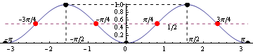
The red dotted points indicate the points of inflection and the black dotted points indicate local extreme values.

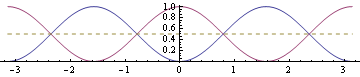
Here is a picture showing the function (blue) and the cosine-squared function (purple) with the dashed line being $y=1/2$. The picture illustrates that $\sin ^{2}x+\cos ^{2}x=1$:

Integration

First antiderivative: using double angle formula

We use the identity:

$\!\sin ^{2}x={\frac {1-\cos(2x)}{2}}$

We can now do the integration:

$\!\int \sin ^{2}x\,dx=\int {\frac {1-\cos(2x)}{2}}\,dx=\int {\frac {1}{2}}\,dx-\int {\frac {\cos(2x)}{2}}\,dx={\frac {x}{2}}-{\frac {\sin(2x)}{4}}+C$

First antiderivative: using integration by parts

We rewrite $\sin ^{2}x=(\sin x)(\sin x)$ and use integration by parts in its recursive version:

$\int \sin ^{2}x\,dx=(\sin x)(-\cos x)-\int (\cos x)(-\cos x)\,dx=-\sin x\cos x+\int \cos ^{2}x\,dx$

We now rewrite $\cos ^{2}x=1-\sin ^{2}x$ and obtain:

$\int \sin ^{2}x\,dx=-\sin x\cos x+\int (1-\sin ^{2}x)\,dx$

Setting $I$ to be a choice of antiderivative so that the above holds without any freely floating constants, we get:

$\!I=-\sin x\cos x+x-I$

Rearranging, we get:

$\!2I=x-\sin x\cos x$

This gives:

$I={\frac {x-\sin x\cos x}{2}}$

So the general antiderivative is:

${\frac {x-\sin x\cos x}{2}}+C$

Using the double angle sine formula $\sin(2x)=2\sin x\cos x$, we can verify that this matches with the preceding answer.

For a given continuous function on a connected set, antiderivatives obtained by different methods must differ by a constant. In some cases, the antiderivatives may be exactly equal, but this is not necessary in general.
See zero derivative implies locally constant

Graph of function with antiderivative

In the picture below, we depict $\sin ^{2}$ (blue) and the function $x\mapsto {\frac {x}{2}}-{\frac {\sin(2x)}{4}}$ (purple). This is the unique antiderivative that takes the value 0 at 0. The other antiderivatives can be obtained by vertically shifting the purple graph:

The black dots correspond to local extreme values for $\sin ^{2}$, and the red dots correspond to points of inflection for the antiderivative. Each black dot is in the same vertical line as a red dot, as we should expect, because points of inflection for the antiderivative correspond to local extreme values for the original function. Further:

• The antiderivative is increasing everywhere because $\sin ^{2}$ is everywhere nonnegative, and is zero only at isolated points.
• The antiderivative is concave up on those intervals where $\sin ^{2}$ is increasing, i.e., intervals of the form $(n\pi ,n\pi +\pi /2)$ as $n$ varies over the integers.
• The antiderivative is concave down on those intervals where $\sin ^{2}$ is decreasing, i.e., intervals of the form $(n\pi +\pi /2,n\pi +\pi )$ as $n$ varies over the integers.

Definite integrals

The $x/2$ part in the antiderivative signifies that the linear part of the antiderivative of $\sin ^{2}$ has slope $1/2$, and this is related to the fact that $\sin ^{2}$ has a mean value of $1/2$ on any interval of length equal to the period. It is in fact clear that the function is a sinusoidal function about $x=1/2$.

Thus, we have:

$\int _{a}^{a+n\pi }\sin ^{2}x\,dx={\frac {n\pi }{2}}$

where $n$ is an integer.

Higher antiderivatives

It is possible to antidifferentiate $\sin ^{2}$ more than once. The $n^{th}$ antiderivative is the sum of a polynomial of degree $n$ and a trigonometric function with a period of $\pi$.

Power series and Taylor series

Computation of power series

We can use the identity:

$\!\sin ^{2}x={\frac {1-\cos(2x)}{2}}$

along with the power series for the cosine function, to find the power series for $\sin ^{2}$.

The power series for the cosine function converges to the function everywhere, and is:

$\!\cos x=1-{\frac {x^{2}}{2!}}+{\frac {x^{4}}{4!}}-{\frac {x^{6}}{6!}}+\dots =\sum _{k=0}^{\infty }{\frac {(-1)^{k}x^{2k}}{(2k)!}}$

The power series for $\cos(2x)$ is:

$\!\cos(2x)=1-{\frac {(2x)^{2}}{2!}}+{\frac {(2x)^{4}}{4!}}-{\frac {(2x)^{6}}{6!}}+\dots =\sum _{k=0}^{\infty }{\frac {(-1)^{k}2^{2k}x^{2k}}{(2k)!}}$

The power series for $1-\cos(2x)$ is:

$\!1-\cos(2x)={\frac {(2x)^{2}}{2!}}-{\frac {(2x)^{4}}{4!}}+{\frac {(2x)^{6}}{6!}}-\dots =\sum _{k=1}^{\infty }{\frac {(-1)^{k-1}2^{2k}x^{2k}}{(2k)!}}$

Dividing by 2, we get the power series for $\sin ^{2}x$:

$\!\sin ^{2}x={\frac {2^{1}x^{2}}{2!}}-{\frac {2^{3}x^{4}}{4!}}+{\frac {2^{5}x^{6}}{6!}}-\dots =\sum _{k=1}^{\infty }{\frac {(-1)^{k-1}2^{2k-1}x^{2k}}{(2k)!}}$

Here's another formulation with the first few terms written more explicitly:

$\!\sin ^{2}x=x^{2}-{\frac {x^{4}}{3}}+{\frac {2x^{6}}{45}}-\dots$

Limit computations

Order of zero

We get the following limit from the power series:

$\!\lim _{x\to 0}{\frac {\sin ^{2}x}{x^{2}}}=1$

Thus, the order of the zero of $\sin ^{2}$ at zero is 2 and the residue is 1.

This limit can be computed in many ways:

Name of method for computing the limit	Details
Simple manipulation, using $\lim _{x\to 0}(\sin x)/x=1$	$\!\lim _{x\to 0}{\frac {\sin ^{2}x}{x^{2}}}=\lim _{x\to 0}\left({\frac {\sin x}{x}}\right)^{2}=\left(\lim _{x\to 0}{\frac {\sin x}{x}}\right)^{2}=1^{2}=1$
Using the L'Hopital rule	$\lim _{x\to 0}{\frac {\sin ^{2}x}{x^{2}}}{\stackrel {*}{=}}\lim _{x\to 0}{\frac {\sin(2x)}{2x}}{\stackrel {*}{=}}{\frac {2\cos(2x)}{2}}=1$
Using the power series	We have $\sin ^{2}x=x^{2}-{\frac {x^{4}}{3}}+\dots$, so we get ${\frac {\sin ^{2}x}{x^{2}}}=1-{\frac {x^{2}}{3}}+\dots$. Taking the limit as $x\to 0$ gives 1.

Higher order limits

We have the limit:

$\!\lim _{x\to 0}{\frac {x^{2}-\sin ^{2}x}{x^{4}}}={\frac {1}{3}}$

This limit can be computed in many ways:

Name of method for computing the limit	Details
Using $\lim _{x\to 0}{\frac {x-\sin x}{x^{3}}}=1/6$ and $\lim _{x\to 0}{\frac {\sin x}{x}}=1$	We have $\lim _{x\to 0}{\frac {x^{2}-\sin ^{2}x}{x^{4}}}=\lim _{x\to 0}{\frac {x-\sin x}{x^{3}}}\cdot {\frac {x+\sin x}{x}}=\lim _{x\to 0}{\frac {x-\sin x}{x^{3}}}\cdot \lim _{x\to 0}{\frac {x+\sin x}{x}}$. The first limit is $1/6$ and the second limit is 2 from the given data. We thus get $(1/6)\cdot 2=1/3$.
Using the L'Hopital rule	$\lim _{x\to 0}{\frac {x^{2}-\sin ^{2}x}{x^{3}}}{\stackrel {*}{=}}\lim _{x\to 0}{\frac {2x-\sin(2x)}{4x^{3}}}{\stackrel {*}{=}}\lim _{x\to 0}{\frac {2-2\cos(2x)}{12x^{2}}}{\stackrel {*}{=}}\lim _{x\to 0}{\frac {4\sin(2x)}{24x}}{\stackrel {*}{=}}\lim _{x\to 0}{\frac {8\cos(2x)}{24}}=1/3$.
Using the power series	We have $\sin ^{2}x=x^{2}-{\frac {x^{4}}{3}}+O(x^{6})$, so ${\frac {x^{2}-\sin ^{2}x}{x^{4}}}={\frac {1}{3}}-O(x^{2})$, so the limit as $x\to 0$ is 1/3.